3. Logistic Regression
Contents
3. Logistic Regression
Introduction
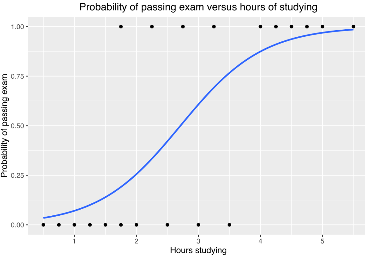
As the amount of available data, the strength of computing power, and the number of algorithmic improvements continue to rise, so does the importance of data science and machine learning. Classification techniques are an essential part of machine learning and data mining applications. Approximately 70% of problems in Data Science are classification problems. There are lots of classification problems that are available, but logistic regression is common and is a useful regression method for solving the binary classification problem. By the end of this tutorial, you’ll have learned about classification in general and the fundamentals of logistic regression in particular, as well as how to implement logistic regression in Python.
In this tutorial, you’ll learn:
What logistic regression is
What logistic regression is used for
How logistic regression works
How to implement logistic regression in Python
What Is Classification?
Supervised machine learning algorithms define models that capture relationships among data. Classification is an area of supervised machine learning that tries to predict which class or category some entity belongs to, based on its features.
For example, you might analyze the employees of some company and try to establish a dependence on the features or variables, such as the level of education, number of years in a current position, age, salary, odds for being promoted, and so on. The set of data related to a single employee is one observation. The features or variables can take one of two forms:
Independent variables, also called inputs or predictors, don’t depend on other features of interest (or at least you assume so for the purpose of the analysis).
Dependent variables, also called outputs or responses, depend on the independent variables.
In the above example where you’re analyzing employees, you might presume the level of education, time in a current position, and age as being mutually independent, and consider them as the inputs. The salary and the odds for promotion could be the outputs that depend on the inputs.
Note: Supervised machine learning algorithms analyze a number of observations and try to mathematically express the dependence between the inputs and outputs. These mathematical representations of dependencies are the models.
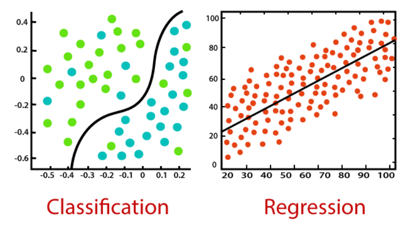
The nature of the dependent variables differentiates regression and classification problems. Regression problems have continuous and usually unbounded outputs. An example is when you’re estimating the salary as a function of experience and education level. On the other hand, classification problems have discrete and finite outputs called classes or categories. For example, predicting if an employee is going to be promoted or not (true or false) is a classification problem.
There are two main types of classification problems:
Binary or binomial classification: exactly two classes to choose between (usually 0 and 1, true and false, or positive and negative)
Multiclass or multinomial classification: three or more classes of the outputs to choose from
If there’s only one input variable, then it’s usually denoted with 𝑥. For more than one input, you’ll commonly see the vector notation 𝐱 = (𝑥₁, …, 𝑥ᵣ), where 𝑟 is the number of the predictors (or independent features). The output variable is often denoted with 𝑦 and takes the values 0 or 1.
When Do You Need Classification?
You can apply classification in many fields of science and technology. For example, text classification algorithms are used to separate legitimate and spam emails, as well as positive and negative comments. You can check out Practical Text Classification With Python and Keras to get some insight into this topic. Other examples involve medical applications, biological classification, credit scoring, and more.
Image recognition tasks are often represented as classification problems. For example, you might ask if an image is depicting a human face or not, or if it’s a mouse or an elephant, or which digit from zero to nine it represents, and so on.
Logistic Regression can be used for various classification problems such as spam detection. Diabetes prediction, if a given customer will purchase a particular product or will they churn another competitor, whether the user will click on a given advertisement link or not, and many more examples are in the bucket.
Logistic Regression is one of the most simple and commonly used Machine Learning algorithms for two-class classification. It is easy to implement and can be used as the baseline for any binary classification problem. Its basic fundamental concepts are also constructive in deep learning. Logistic regression describes and estimates the relationship between one dependent binary variable and independent variables.
Logistic Regression Overview
Logistic Regression is a Machine Learning classification algorithm that is used to predict the probability of a categorical dependent variable. In logistic regression, the dependent variable is a binary variable that contains data coded as 1 (yes, success, etc.) or 0 (no, failure, etc.). In other words, the logistic regression model predicts P(Y=1) as a function of X.
Wiki Logistic Regression
Tutorial Introduction to Logistic Regression
Differences between Linear Regression and Logistic Regression
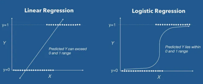
The relation between Linear and Logistic Regression is the fact that they use labeled datasets to make predictions. However, the main difference between them is how they are being used. Linear Regression is used to solve Regression problems whereas Logistic Regression is used to solve Classification problems.
Classification is about predicting a label, by identifying which category an object belongs to based on different parameters.
Regression is about predicting a continuous output, by finding the correlations between dependent and independent variables.
Review of Linear Regression
Linear Regression is known as one of the simplest Machine learning algorithms that branch from Supervised Learning and is primarily used to solve regression problems.
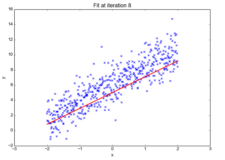
The use of Linear Regression is to make predictions on continuous dependent variables with the assistance and knowledge from independent variables. The overall goal of Linear Regression is to find the line of best fit, which can accurately predict the output for continuous dependent variables. Examples of continuous values are house prices, age, and salary.
Simple Linear Regression is a regression model that estimates the relationship between one single independent variable and one dependent variable using a straight line. If there are more than two independent variables, we then call this Multiple Linear Regression.
Using the strategy of the line of best fits helps us to understand the relationship between the dependent and independent variable; which should be of linear nature.
The Formula for Linear Regression
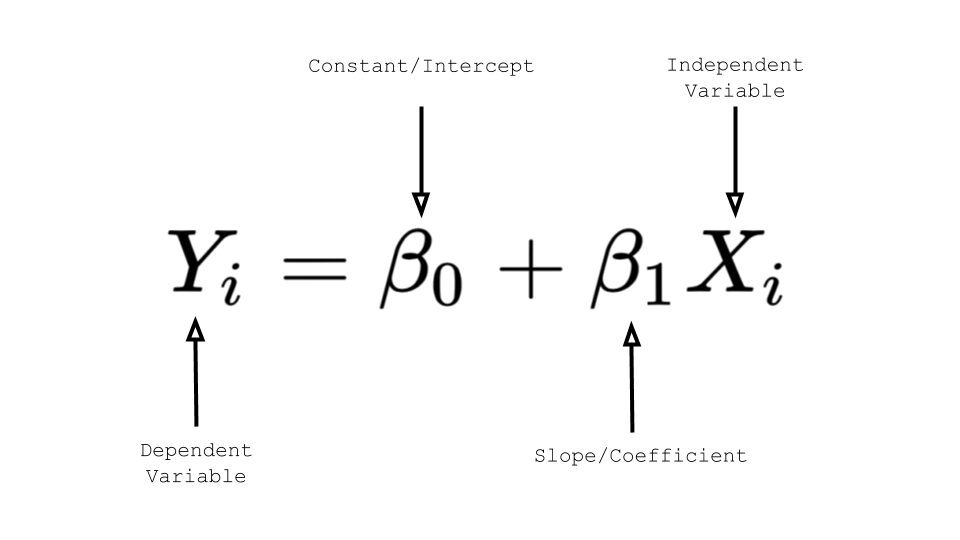
If you remember high school Mathematics, you will remember the formula: y = mx + b and represents the slope-intercept of a straight line. ‘y’ and ‘x’ represent variables, ‘m’ describes the slope of the line and ‘b’ describe the y-intercept, where the line crosses the y-axis.
For Linear Regression, ‘y’ represents the dependent variable, ‘x’ represents the independent variable, 𝜷0 represents the y-intercept and 𝜷1 represents the slope, which describes the relationship between the independent variable and the dependent variable
A regression line is obtained which will give the minimum error. To do that he needs to make a line that is closest to as many points as possible.
Where ‘β1’ is the slope and ‘βo’ is the y-intercept similar to the equation of a line. The values ‘β1’ and ‘βo’ must be chosen so that they minimize the error. To check the error we have to calculate the sum of squared error and tune the parameters to try to reduce the error.
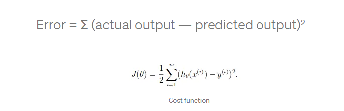
Key:
Y(predicted) is also called the hypothesis function.
J(θ) is the cost function which can also be called the error function. Our main goal is to minimize the value of the cost.
y(i) is the predicted output.
hθ(x(i)) is called the hypothesis function which is basically the Y(predicted) value.
Now the question arises, how do we reduce the error value. Well, this can be done by using Gradient Descent. The main goal of Gradient descent is to minimize the cost value. i.e. min J(θo, θ1)
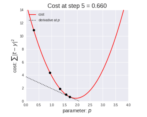
Gradient descent has an analogy in which we have to imagine ourselves at the top of a mountain valley and left stranded and blindfolded, our objective is to reach the bottom of the hill. Feeling the slope of the terrain around you is what everyone would do. Well, this action is analogous to calculating the gradient descent, and taking a step is analogous to one iteration of the update to the parameters.
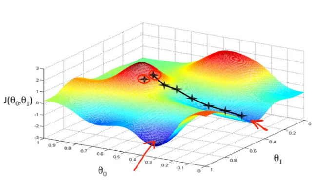
Choosing a perfect learning rate is a very important task as it depends on how large of a step we take downhill during each iteration. If we take too large of a step, we may step over the minimum. However, if we take small steps, it will require many iterations to arrive at the minimum.
Logistic Regression
Logistic Regression is also a very popular Machine Learning algorithm that branches off Supervised Learning. Logistic Regression is mainly used for Classification tasks.
An example of Logistic Regression predicting whether it will rain today or not, by using 0 or 1, yes or no, or true and false.
The use of Logistic Regression is to predict the categorical dependent variable with the assistance and knowledge of independent variables. The overall aim of Logistic Regression is to classify outputs, which can only be between 0 and 1.
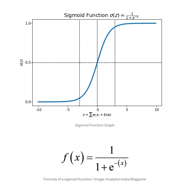
In Logistic Regression the weighted sum of inputs is passed through an activation function called Sigmoid Function which maps values between 0 and 1.
The Logistic Regression uses a more complex cost function, this cost function can be defined as the ‘Sigmoid function’ or also known as the ‘logistic function’ instead of a linear function.
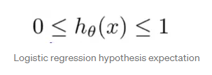
The hypothesis of logistic regression tends it to limit the cost function between 0 and 1. Therefore linear functions fail to represent it as it can have a value greater than 1 or less than 0 which is not possible as per the hypothesis of logistic regression.
In order to map predicted values to probabilities, we use the Sigmoid function. The function maps any real value into another value between 0 and 1. In machine learning, we use sigmoid to map predictions to probabilities.
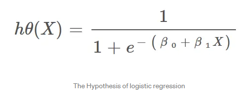
Hypothesis Representation When using linear regression we used a formula of the hypothesis i.e.
hΘ(x) = β₀ + β₁X
For logistic regression we are going to modify it a little bit i.e.
σ(Z) = σ(β₀ + β₁X)
We have expected that our hypothesis will give values between 0 and 1.
Z = β₀ + β₁X
hΘ(x) = sigmoid(Z)
The final hypothesis formula
We expect our classifier to give us a set of outputs or classes based on probability when we pass the inputs through a prediction function and returns a probability score between 0 and 1.
For Example, We have 2 classes, let’s take them like cats and dogs(1 — dog , 0 — cats). We basically decide with a threshold value above which we classify values into Class 1 and of the value goes below the threshold then we classify it in Class 2.
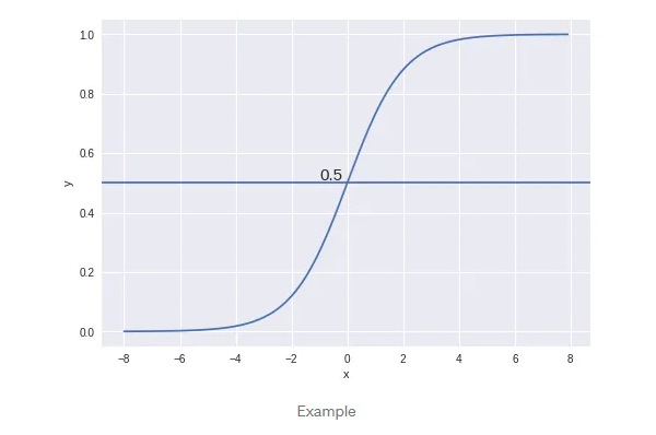
As shown in the above graph we have chosen the threshold as 0.5, if the prediction function returned a value of 0.7 then we would classify this observation as Class 1(DOG). If our prediction returned a value of 0.2 then we would classify the observation as Class 2(CAT).
We learnt about the cost function J(θ) in the Linear regression, the cost function represents optimization objective i.e. we create a cost function and minimize it so that we can develop an accurate model with minimum error.
The Cost Function of a Linear Regression is root mean squared error or also known as mean squared error (MSE).
MSE measures the average squared difference between an observation’s actual and predicted values. The cost will be outputted as a single number which is associated with our current set of weights. The reason we use Cost Function is to improve the accuracy of the model
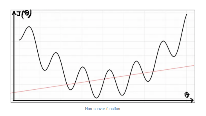
If we try to use the cost function of the linear regression in ‘Logistic Regression’ then it would be of no use as it would end up being a non-convex function with many local minimums, in which it would be very difficult to minimize the cost value and find the global minimum.
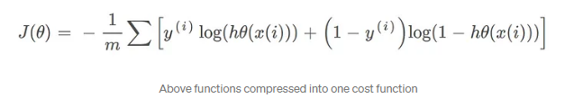
For logistic regression, the Cost function is defined as:
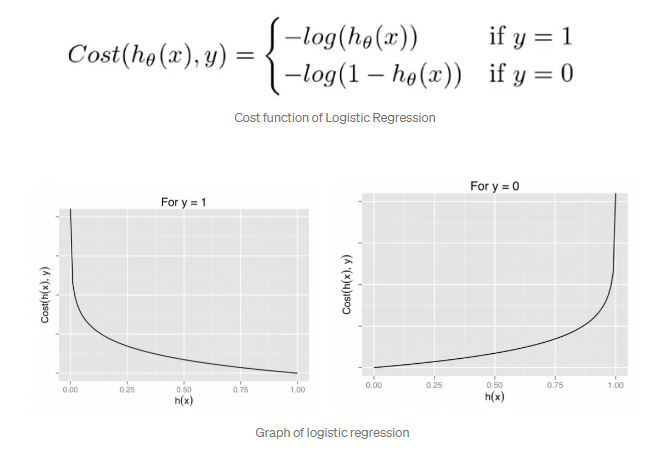
The above two functions can be compressed into a single function i.e.
Gradient Descent
Now the question arises, how do we reduce the cost value. Well, this can be done by using Gradient Descent. The main goal of Gradient descent is to minimize the cost value. i.e. min J(θ).
Now to minimize our cost function we need to run the gradient descent function on each parameter i.e.
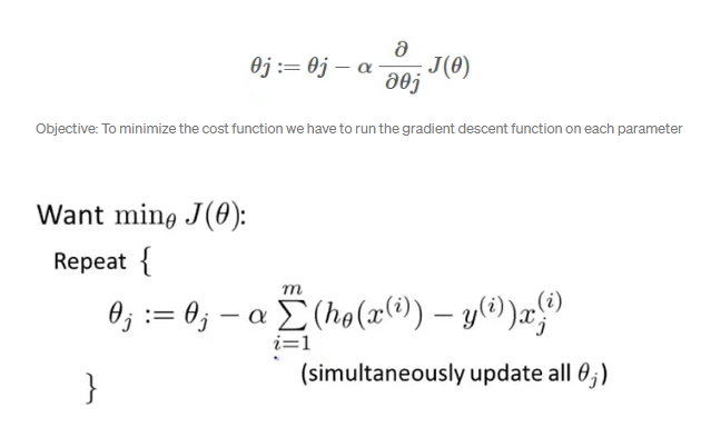
Gradient descent has an analogy in which we have to imagine ourselves at the top of a mountain valley and left stranded and blindfolded, our objective is to reach the bottom of the hill. Feeling the slope of the terrain around you is what everyone would do. Well, this action is analogous to calculating the gradient descent, and taking a step is analogous to one iteration of the update to the parameters.
Math Tutorial for Logistic Regression Logistic Regression
Math Tutorial for Linear Regression Linear Regression
Environment setup
import platform

print(f"Python version: {platform.python_version()}")
assert platform.python_version_tuple() >= ("3", "6")

import numpy as np
import matplotlib
import matplotlib.pyplot as plt
from matplotlib.colors import ListedColormap
import seaborn as sns
Python version: 3.7.11
D:\ProgramData\Anaconda3\lib\site-packages\pandas\compat\_optional.py:138: UserWarning: Pandas requires version '2.7.0' or newer of 'numexpr' (version '2.6.9' currently installed).
  warnings.warn(msg, UserWarning)
# Setup plots
%matplotlib inline
plt.rcParams["figure.figsize"] = 10, 8
%config InlineBackend.figure_format = 'retina'
sns.set()
import sklearn

print(f"scikit-learn version: {sklearn.__version__}")
assert sklearn.__version__ >= "0.20"

from sklearn.datasets import make_classification, make_blobs
from sklearn.linear_model import SGDClassifier, LogisticRegression
from sklearn.metrics import classification_report
scikit-learn version: 0.20.3
def plot_data(x, y):
    """Plot some 2D data"""

    fig, ax = plt.subplots()
    scatter = ax.scatter(x[:, 0], x[:, 1], c=y, s=40, cmap=plt.cm.RdYlBu)
    legend1 = ax.legend(*scatter.legend_elements(),
                    loc="lower right", title="Classes")
    ax.add_artist(legend1)
    plt.xlim((min(x[:, 0]) - 0.1, max(x[:, 0]) + 0.1))
    plt.ylim((min(x[:, 1]) - 0.1, max(x[:, 1]) + 0.1))


def plot_decision_boundary(pred_func, x, y, figure=None):
    """Plot a decision boundary"""

    if figure is None:  # If no figure is given, create a new one
        plt.figure()
    # Set min and max values and give it some padding
    x_min, x_max = x[:, 0].min() - 0.5, x[:, 0].max() + 0.5
    y_min, y_max = x[:, 1].min() - 0.5, x[:, 1].max() + 0.5
    h = 0.01
    # Generate a grid of points with distance h between them
    xx, yy = np.meshgrid(np.arange(x_min, x_max, h), np.arange(y_min, y_max, h))
    # Predict the function value for the whole grid
    Z = pred_func(np.c_[xx.ravel(), yy.ravel()])
    Z = Z.reshape(xx.shape)
    # Plot the contour and training examples
    plt.contourf(xx, yy, Z, cmap=plt.cm.Spectral)
    cm_bright = ListedColormap(["#FF0000", "#00FF00", "#0000FF"])
    plt.scatter(x[:, 0], x[:, 1], c=y, s=40, cmap=plt.cm.RdYlBu, alpha=0.8)
Binary classification
Problem formulation
Logistic regression is a classification algorithm used to estimate the probability that a data sample belongs to a particular class.
A logistic regression model computes a weighted sum of the input features (plus a bias term), then applies the logistic function to this sum in order to output a probability.
The function output is thresholded to form the model’s prediction:
\(0\) if \(y' \lt 0.5\)
\(1\) if \(y' \geqslant 0.5\)
Loss function: Binary Crossentropy (log loss)
See loss definition for details.
Model training
No analytical solution because of the non-linear \(\sigma()\) function: gradient descent is the only option.
Since the loss function is convex, GD (with the right hyperparameters) is guaranteed to find the global loss minimum.
Different GD optimizers exist: newton-cg, l-bfgs, sag… Stochastic gradient descent is another possibility, efficient for large numbers of samples and features.
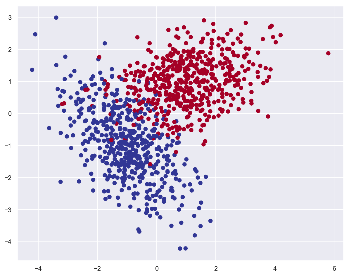
Example: classify planar data
# Generate 2 classes of linearly separable data
x_train, y_train = make_classification(
    n_samples=1000,
    n_features=2,
    n_redundant=0,
    n_informative=2,
    random_state=26,
    n_clusters_per_class=1,
)
plot_data(x_train, y_train)
---------------------------------------------------------------------------
AttributeError                            Traceback (most recent call last)
<ipython-input-5-1b1108a63e4a> in <module>
      8     n_clusters_per_class=1,
      9 )
---> 10 plot_data(x_train, y_train)

<ipython-input-4-b2991d7dc072> in plot_data(x, y)
      4     fig, ax = plt.subplots()
      5     scatter = ax.scatter(x[:, 0], x[:, 1], c=y, s=40, cmap=plt.cm.RdYlBu)
----> 6     legend1 = ax.legend(*scatter.legend_elements(),
      7                     loc="lower right", title="Classes")
      8     ax.add_artist(legend1)

AttributeError: 'PathCollection' object has no attribute 'legend_elements'
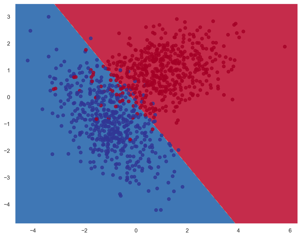
# Create a Logistic Regression model based on stochastic gradient descent
# Alternative: using the LogisticRegression class which implements many GD optimizers
lr_model = SGDClassifier(loss="log")

# Train the model
lr_model.fit(x_train, y_train)

print(f"Model weights: {lr_model.coef_}, bias: {lr_model.intercept_}")
Model weights: [[-2.96719034 -2.55668143]], bias: [-0.57585284]
# Print report with classification metrics
print(classification_report(y_train, lr_model.predict(x_train)))
              precision    recall  f1-score   support

           0       0.96      0.92      0.94       502
           1       0.92      0.96      0.94       498

    accuracy                           0.94      1000
   macro avg       0.94      0.94      0.94      1000
weighted avg       0.94      0.94      0.94      1000
# Plot decision boundary
plot_decision_boundary(lambda x: lr_model.predict(x), x_train, y_train)
Multivariate regression
Problem formulation
Multivariate regression, also called softmax regression, is a generalization of logistic regression for multiclass classification.
A softmax regression model computes the scores \(s_k(\pmb{x})\) for each class \(k\), then estimates probabilities for each class by applying the softmax function to compute a probability distribution.
For a sample \(\pmb{x}^{(i)}\), the model predicts the class \(k\) that has the highest probability.
Each class \(k\) has its own parameter vector \(\pmb{\theta}^{(k)}\).
Model output
\(\pmb{y}^{(i)}\) (ground truth): binary vector of \(K\) values. \(y^{(i)}_k\) is equal to 1 if the \(i\)th sample’s class corresponds to \(k\), 0 otherwise.
\(\pmb{y}'^{(i)}\): probability vector of \(K\) values, computed by the model. \(y'^{(i)}_k\) represents the probability that the \(i\)th sample belongs to class \(k\).
Loss function: Categorical Crossentropy
See loss definition for details.
Model training
Via gradient descent:
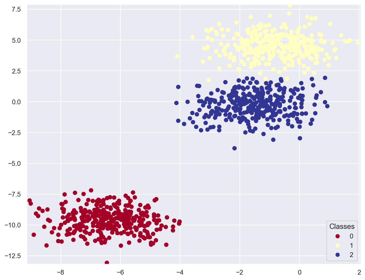
Example: classify multiclass planar data
# Generate 3 classes of linearly separable data
x_train_multi, y_train_multi = make_blobs(n_samples=1000, n_features=2, centers=3, random_state=11)

plot_data(x_train_multi, y_train_multi)
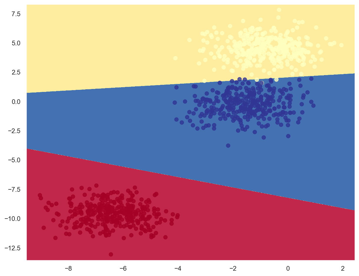
# Create a Logistic Regression model based on stochastic gradient descent
# Alternative: using LogisticRegression(multi_class="multinomial") which implements SR
lr_model_multi = SGDClassifier(loss="log")

# Train the model
lr_model_multi.fit(x_train_multi, y_train_multi)

print(f"Model weights: {lr_model_multi.coef_}, bias: {lr_model_multi.intercept_}")
Model weights: [[ -5.76624648 -17.43149458]
 [ -1.27339599  19.17812979]
 [  1.5231193   -0.91647832]], bias: [-133.15588019  -38.36388245    2.53712564]
# Print report with classification metrics
print(classification_report(y_train_multi, lr_model_multi.predict(x_train_multi)))
              precision    recall  f1-score   support

           0       1.00      1.00      1.00       334
           1       0.99      0.99      0.99       333
           2       0.99      0.99      0.99       333

    accuracy                           0.99      1000
   macro avg       0.99      0.99      0.99      1000
weighted avg       1.00      0.99      0.99      1000
# Plot decision boundaries
plot_decision_boundary(lambda x: lr_model_multi.predict(x), x_train_multi, y_train_multi)
Titanic Disaster Survival Using Logistic Regression
#import libraries
import pandas as pd
import numpy as np
import seaborn as sns
import matplotlib.pyplot as plt
Load the Data
#load data
titanic_data=pd.read_csv('titanic_train.csv')
len(titanic_data)
891
View the data using head function which returns top rows
titanic_data.head()
| PassengerId | Survived | Pclass | Name | Sex | Age | SibSp | Parch | Ticket | Fare | Cabin | Embarked | |
|---|---|---|---|---|---|---|---|---|---|---|---|---|
| 0 | 1 | 0 | 3 | Braund, Mr. Owen Harris | male | 22.0 | 1 | 0 | A/5 21171 | 7.2500 | NaN | S |
| 1 | 2 | 1 | 1 | Cumings, Mrs. John Bradley (Florence Briggs Th... | female | 38.0 | 1 | 0 | PC 17599 | 71.2833 | C85 | C |
| 2 | 3 | 1 | 3 | Heikkinen, Miss. Laina | female | 26.0 | 0 | 0 | STON/O2. 3101282 | 7.9250 | NaN | S |
| 3 | 4 | 1 | 1 | Futrelle, Mrs. Jacques Heath (Lily May Peel) | female | 35.0 | 1 | 0 | 113803 | 53.1000 | C123 | S |
| 4 | 5 | 0 | 3 | Allen, Mr. William Henry | male | 35.0 | 0 | 0 | 373450 | 8.0500 | NaN | S |
titanic_data.index
RangeIndex(start=0, stop=891, step=1)
titanic_data.columns
Index(['PassengerId', 'Survived', 'Pclass', 'Name', 'Sex', 'Age', 'SibSp',
       'Parch', 'Ticket', 'Fare', 'Cabin', 'Embarked'],
      dtype='object')
titanic_data.info()
<class 'pandas.core.frame.DataFrame'>
RangeIndex: 891 entries, 0 to 890
Data columns (total 12 columns):
 #   Column       Non-Null Count  Dtype
---  ------       --------------  -----
 0   PassengerId  891 non-null    int64
 1   Survived     891 non-null    int64
 2   Pclass       891 non-null    int64
 3   Name         891 non-null    object
 4   Sex          891 non-null    object
 5   Age          714 non-null    float64
 6   SibSp        891 non-null    int64
 7   Parch        891 non-null    int64
 8   Ticket       891 non-null    object
 9   Fare         891 non-null    float64
 10  Cabin        204 non-null    object
 11  Embarked     889 non-null    object
dtypes: float64(2), int64(5), object(5)
memory usage: 83.7+ KB
titanic_data.dtypes
PassengerId      int64
Survived         int64
Pclass           int64
Name            object
Sex             object
Age            float64
SibSp            int64
Parch            int64
Ticket          object
Fare           float64
Cabin           object
Embarked        object
dtype: object
titanic_data.describe()
| PassengerId | Survived | Pclass | Age | SibSp | Parch | Fare | |
|---|---|---|---|---|---|---|---|
| count | 891.000000 | 891.000000 | 891.000000 | 714.000000 | 891.000000 | 891.000000 | 891.000000 |
| mean | 446.000000 | 0.383838 | 2.308642 | 29.699118 | 0.523008 | 0.381594 | 32.204208 |
| std | 257.353842 | 0.486592 | 0.836071 | 14.526497 | 1.102743 | 0.806057 | 49.693429 |
| min | 1.000000 | 0.000000 | 1.000000 | 0.420000 | 0.000000 | 0.000000 | 0.000000 |
| 25% | 223.500000 | 0.000000 | 2.000000 | 20.125000 | 0.000000 | 0.000000 | 7.910400 |
| 50% | 446.000000 | 0.000000 | 3.000000 | 28.000000 | 0.000000 | 0.000000 | 14.454200 |
| 75% | 668.500000 | 1.000000 | 3.000000 | 38.000000 | 1.000000 | 0.000000 | 31.000000 |
| max | 891.000000 | 1.000000 | 3.000000 | 80.000000 | 8.000000 | 6.000000 | 512.329200 |
Explaining Dataset
survival : Survival 0 = No, 1 = Yes
pclass : Ticket class 1 = 1st, 2 = 2nd, 3 = 3rd
sex : Sex
Age : Age in years
sibsp : Number of siblings / spouses aboard the Titanic
parch # of parents / children aboard the Titanic
ticket : Ticket number fare Passenger fare cabin Cabin number
embarked : Port of Embarkation C = Cherbourg, Q = Queenstown, S = Southampton
Data Analysis
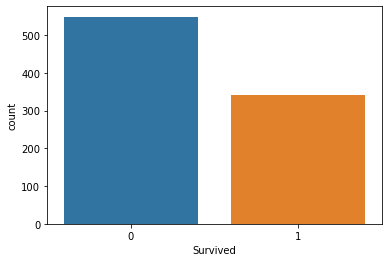
Import Seaborn for visually analysing the data, Find out how many survived vs Died using countplot method of seaboarn
#countplot of subrvived vs not survived
sns.countplot(x='Survived',data=titanic_data)
<AxesSubplot:xlabel='Survived', ylabel='count'>
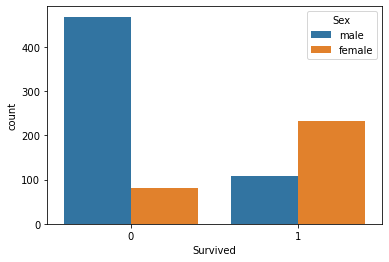
Male vs Female Survival
#Male vs Female Survived?
sns.countplot(x='Survived',data=titanic_data,hue='Sex')
<AxesSubplot:xlabel='Survived', ylabel='count'>
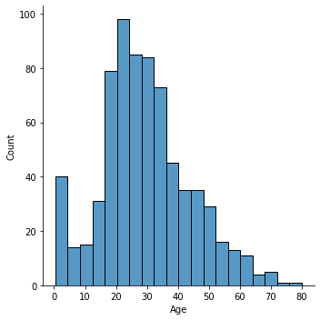
**See age group of passengeres travelled **
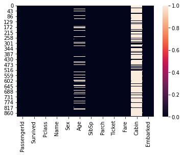
Note: We will use displot method to see the histogram. However some records does not have age hence the method will throw an error. In order to avoid that we will use dropna method to eliminate null values from graph
#Check for null
titanic_data.isna()
| PassengerId | Survived | Pclass | Name | Sex | Age | SibSp | Parch | Ticket | Fare | Cabin | Embarked | |
|---|---|---|---|---|---|---|---|---|---|---|---|---|
| 0 | False | False | False | False | False | False | False | False | False | False | True | False |
| 1 | False | False | False | False | False | False | False | False | False | False | False | False |
| 2 | False | False | False | False | False | False | False | False | False | False | True | False |
| 3 | False | False | False | False | False | False | False | False | False | False | False | False |
| 4 | False | False | False | False | False | False | False | False | False | False | True | False |
| ... | ... | ... | ... | ... | ... | ... | ... | ... | ... | ... | ... | ... |
| 886 | False | False | False | False | False | False | False | False | False | False | True | False |
| 887 | False | False | False | False | False | False | False | False | False | False | False | False |
| 888 | False | False | False | False | False | True | False | False | False | False | True | False |
| 889 | False | False | False | False | False | False | False | False | False | False | False | False |
| 890 | False | False | False | False | False | False | False | False | False | False | True | False |
891 rows × 12 columns
#Check how many values are null
titanic_data.isna().sum()
PassengerId      0
Survived         0
Pclass           0
Name             0
Sex              0
Age            177
SibSp            0
Parch            0
Ticket           0
Fare             0
Cabin          687
Embarked         2
dtype: int64
#Visualize null values
sns.heatmap(titanic_data.isna())
<AxesSubplot:>
#find the % of null values in age column
(titanic_data['Age'].isna().sum()/len(titanic_data['Age']))*100
19.865319865319865
#find the % of null values in cabin column
(titanic_data['Cabin'].isna().sum()/len(titanic_data['Cabin']))*100
77.10437710437711
#find the distribution for the age column
sns.displot(x='Age',data=titanic_data)
<seaborn.axisgrid.FacetGrid at 0x1509b6c8a30>
Data Cleaning
Fill the missing values
we will fill the missing values for age. In order to fill missing values we use fillna method.
For now we will fill the missing age by taking average of all age
#fill age column
titanic_data['Age'].fillna(titanic_data['Age'].mean(),inplace=True)
We can verify that no more null data exist
we will examine data by isnull mehtod which will return nothing
#verify null value
titanic_data['Age'].isna().sum()
0
Alternatively we will visualise the null value using heatmap
we will use heatmap method by passing only records which are null.
#visualize null values
sns.heatmap(titanic_data.isna())
<AxesSubplot:>
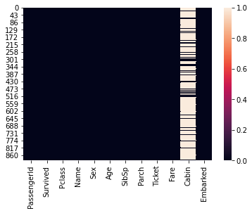
We can see cabin column has a number of null values, as such we can not use it for prediction. Hence we will drop it
#Drop cabin column
titanic_data.drop('Cabin',axis=1,inplace=True)
#see the contents of the data
titanic_data.head()
| PassengerId | Survived | Pclass | Name | Sex | Age | SibSp | Parch | Ticket | Fare | Embarked | |
|---|---|---|---|---|---|---|---|---|---|---|---|
| 0 | 1 | 0 | 3 | Braund, Mr. Owen Harris | male | 22.0 | 1 | 0 | A/5 21171 | 7.2500 | S |
| 1 | 2 | 1 | 1 | Cumings, Mrs. John Bradley (Florence Briggs Th... | female | 38.0 | 1 | 0 | PC 17599 | 71.2833 | C |
| 2 | 3 | 1 | 3 | Heikkinen, Miss. Laina | female | 26.0 | 0 | 0 | STON/O2. 3101282 | 7.9250 | S |
| 3 | 4 | 1 | 1 | Futrelle, Mrs. Jacques Heath (Lily May Peel) | female | 35.0 | 1 | 0 | 113803 | 53.1000 | S |
| 4 | 5 | 0 | 3 | Allen, Mr. William Henry | male | 35.0 | 0 | 0 | 373450 | 8.0500 | S |
Preaparing Data for Model
No we will require to convert all non-numerical columns to numeric. Please note this is required for feeding data into model. Lets see which columns are non numeric info describe method
#Check for the non-numeric column
titanic_data.info()
<class 'pandas.core.frame.DataFrame'>
RangeIndex: 891 entries, 0 to 890
Data columns (total 11 columns):
 #   Column       Non-Null Count  Dtype
---  ------       --------------  -----
 0   PassengerId  891 non-null    int64
 1   Survived     891 non-null    int64
 2   Pclass       891 non-null    int64
 3   Name         891 non-null    object
 4   Sex          891 non-null    object
 5   Age          891 non-null    float64
 6   SibSp        891 non-null    int64
 7   Parch        891 non-null    int64
 8   Ticket       891 non-null    object
 9   Fare         891 non-null    float64
 10  Embarked     889 non-null    object
dtypes: float64(2), int64(5), object(4)
memory usage: 76.7+ KB
titanic_data.dtypes
PassengerId      int64
Survived         int64
Pclass           int64
Name            object
Sex             object
Age            float64
SibSp            int64
Parch            int64
Ticket          object
Fare           float64
Embarked        object
dtype: object
We can see, Name, Sex, Ticket and Embarked are non-numerical.It seems Name,Embarked and Ticket number are not useful for Machine Learning Prediction hence we will eventually drop it. For Now we would convert Sex Column to dummies numerical values****
#convert sex column to numerical values
gender=pd.get_dummies(titanic_data['Sex'],drop_first=True)
titanic_data['Gender']=gender
titanic_data.head()
| PassengerId | Survived | Pclass | Name | Sex | Age | SibSp | Parch | Ticket | Fare | Embarked | Gender | |
|---|---|---|---|---|---|---|---|---|---|---|---|---|
| 0 | 1 | 0 | 3 | Braund, Mr. Owen Harris | male | 22.0 | 1 | 0 | A/5 21171 | 7.2500 | S | 1 |
| 1 | 2 | 1 | 1 | Cumings, Mrs. John Bradley (Florence Briggs Th... | female | 38.0 | 1 | 0 | PC 17599 | 71.2833 | C | 0 |
| 2 | 3 | 1 | 3 | Heikkinen, Miss. Laina | female | 26.0 | 0 | 0 | STON/O2. 3101282 | 7.9250 | S | 0 |
| 3 | 4 | 1 | 1 | Futrelle, Mrs. Jacques Heath (Lily May Peel) | female | 35.0 | 1 | 0 | 113803 | 53.1000 | S | 0 |
| 4 | 5 | 0 | 3 | Allen, Mr. William Henry | male | 35.0 | 0 | 0 | 373450 | 8.0500 | S | 1 |
#drop the columns which are not required
titanic_data.drop(['Name','Sex','Ticket','Embarked'],axis=1,inplace=True)
titanic_data.head()
| PassengerId | Survived | Pclass | Age | SibSp | Parch | Fare | Gender | |
|---|---|---|---|---|---|---|---|---|
| 0 | 1 | 0 | 3 | 22.0 | 1 | 0 | 7.2500 | 1 |
| 1 | 2 | 1 | 1 | 38.0 | 1 | 0 | 71.2833 | 0 |
| 2 | 3 | 1 | 3 | 26.0 | 0 | 0 | 7.9250 | 0 |
| 3 | 4 | 1 | 1 | 35.0 | 1 | 0 | 53.1000 | 0 |
| 4 | 5 | 0 | 3 | 35.0 | 0 | 0 | 8.0500 | 1 |
#Seperate Dependent and Independent variables
x=titanic_data[['PassengerId','Pclass','Age','SibSp','Parch','Fare','Gender']]
y=titanic_data['Survived']
y
0      0
1      1
2      1
3      1
4      0
      ..
886    0
887    1
888    0
889    1
890    0
Name: Survived, Length: 891, dtype: int64
Data Modelling
Building Model using Logestic Regression
Build the model
#import train test split method
from sklearn.model_selection import train_test_split
#train test split
x_train, x_test, y_train, y_test = train_test_split(x, y, test_size=0.33, random_state=42)
#import Logistic Regression
from sklearn.linear_model import LogisticRegression
#Fit Logistic Regression
lr=LogisticRegression()
lr.fit(x_train,y_train)
C:\Users\gggg\anaconda3\lib\site-packages\sklearn\linear_model\_logistic.py:762: ConvergenceWarning: lbfgs failed to converge (status=1):
STOP: TOTAL NO. of ITERATIONS REACHED LIMIT.

Increase the number of iterations (max_iter) or scale the data as shown in:
    https://scikit-learn.org/stable/modules/preprocessing.html
Please also refer to the documentation for alternative solver options:
    https://scikit-learn.org/stable/modules/linear_model.html#logistic-regression
  n_iter_i = _check_optimize_result(
LogisticRegression()
#predict
predict=lr.predict(x_test)
Testing
See how our model is performing
#print confusion matrix
from sklearn.metrics import confusion_matrix
pd.DataFrame(confusion_matrix(y_test,predict),columns=['Predicted No','Predicted Yes'],index=['Actual No','Actual Yes'])
| Predicted No | Predicted Yes | |
|---|---|---|
| Actual No | 151 | 24 |
| Actual Yes | 37 | 83 |
Classification Performance
Binary classification has four possible types of results:
True negatives: correctly predicted negatives (zeros)
True positives: correctly predicted positives (ones)
False negatives: incorrectly predicted negatives (zeros)
False positives: incorrectly predicted positives (ones) You usually evaluate the performance of your classifier by comparing the actual and predicted outputsand counting the correct and incorrect predictions.
The most straightforward indicator of classification accuracy is the ratio of the number of correct predictions to the total number of predictions (or observations). Other indicators of binary classifiers include the following:
The positive predictive value is the ratio of the number of true positives to the sum of the numbers of true and false positives.
The negative predictive value is the ratio of the number of true negatives to the sum of the numbers of true and false negatives.
The sensitivity (also known as recall or true positive rate) is the ratio of the number of true positives to the number of actual positives.
The specificity (or true negative rate) is the ratio of the number of true negatives to the number of actual negatives.
#import classification report
from sklearn.metrics import classification_report
print(classification_report(y_test,predict))
              precision    recall  f1-score   support

           0       0.80      0.86      0.83       175
           1       0.78      0.69      0.73       120

    accuracy                           0.79       295
   macro avg       0.79      0.78      0.78       295
weighted avg       0.79      0.79      0.79       295
Precision is fine considering Model Selected and Available Data. Accuracy can be increased by further using more features (which we dropped earlier) and/or by using other model
Note:
Precision : Precision is the ratio of correctly predicted positive observations to the total predicted positive observations
Recall : Recall is the ratio of correctly predicted positive observations to the all observations in actual class
F1 score - F1 Score is the weighted average of Precision and Recall.