Logistic Regression
Contents
Logistic Regression
Environment setup
import platform

print(f"Python version: {platform.python_version()}")
assert platform.python_version_tuple() >= ("3", "6")

import numpy as np
import matplotlib
import matplotlib.pyplot as plt
from matplotlib.colors import ListedColormap
import seaborn as sns
Python version: 3.7.11
D:\ProgramData\Anaconda3\lib\site-packages\pandas\compat\_optional.py:138: UserWarning: Pandas requires version '2.7.0' or newer of 'numexpr' (version '2.6.9' currently installed).
  warnings.warn(msg, UserWarning)
# Setup plots
%matplotlib inline
plt.rcParams["figure.figsize"] = 10, 8
%config InlineBackend.figure_format = 'retina'
sns.set()
import sklearn

print(f"scikit-learn version: {sklearn.__version__}")
assert sklearn.__version__ >= "0.20"

from sklearn.datasets import make_classification, make_blobs
from sklearn.linear_model import SGDClassifier, LogisticRegression
from sklearn.metrics import classification_report
scikit-learn version: 0.20.3
def plot_data(x, y):
    """Plot some 2D data"""

    fig, ax = plt.subplots()
    scatter = ax.scatter(x[:, 0], x[:, 1], c=y, s=40, cmap=plt.cm.RdYlBu)
    legend1 = ax.legend(*scatter.legend_elements(),
                    loc="lower right", title="Classes")
    ax.add_artist(legend1)
    plt.xlim((min(x[:, 0]) - 0.1, max(x[:, 0]) + 0.1))
    plt.ylim((min(x[:, 1]) - 0.1, max(x[:, 1]) + 0.1))


def plot_decision_boundary(pred_func, x, y, figure=None):
    """Plot a decision boundary"""

    if figure is None:  # If no figure is given, create a new one
        plt.figure()
    # Set min and max values and give it some padding
    x_min, x_max = x[:, 0].min() - 0.5, x[:, 0].max() + 0.5
    y_min, y_max = x[:, 1].min() - 0.5, x[:, 1].max() + 0.5
    h = 0.01
    # Generate a grid of points with distance h between them
    xx, yy = np.meshgrid(np.arange(x_min, x_max, h), np.arange(y_min, y_max, h))
    # Predict the function value for the whole grid
    Z = pred_func(np.c_[xx.ravel(), yy.ravel()])
    Z = Z.reshape(xx.shape)
    # Plot the contour and training examples
    plt.contourf(xx, yy, Z, cmap=plt.cm.Spectral)
    cm_bright = ListedColormap(["#FF0000", "#00FF00", "#0000FF"])
    plt.scatter(x[:, 0], x[:, 1], c=y, s=40, cmap=plt.cm.RdYlBu, alpha=0.8)
Binary classification
Problem formulation
Logistic regression is a classification algorithm used to estimate the probability that a data sample belongs to a particular class.
A logistic regression model computes a weighted sum of the input features (plus a bias term), then applies the logistic function to this sum in order to output a probability.
The function output is thresholded to form the model’s prediction:
\(0\) if \(y' \lt 0.5\)
\(1\) if \(y' \geqslant 0.5\)
Loss function: Binary Crossentropy (log loss)
See loss definition for details.
Model training
No analytical solution because of the non-linear \(\sigma()\) function: gradient descent is the only option.
Since the loss function is convex, GD (with the right hyperparameters) is guaranteed to find the global loss minimum.
Different GD optimizers exist: newton-cg, l-bfgs, sag… Stochastic gradient descent is another possibility, efficient for large numbers of samples and features.
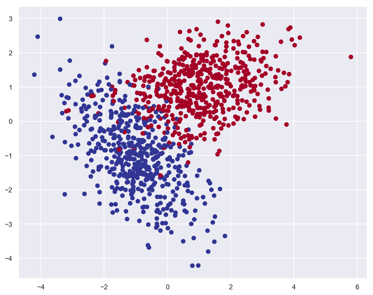
Example: classify planar data
# Generate 2 classes of linearly separable data
x_train, y_train = make_classification(
    n_samples=1000,
    n_features=2,
    n_redundant=0,
    n_informative=2,
    random_state=26,
    n_clusters_per_class=1,
)
plot_data(x_train, y_train)
---------------------------------------------------------------------------
AttributeError                            Traceback (most recent call last)
<ipython-input-5-1b1108a63e4a> in <module>
      8     n_clusters_per_class=1,
      9 )
---> 10 plot_data(x_train, y_train)

<ipython-input-4-b2991d7dc072> in plot_data(x, y)
      4     fig, ax = plt.subplots()
      5     scatter = ax.scatter(x[:, 0], x[:, 1], c=y, s=40, cmap=plt.cm.RdYlBu)
----> 6     legend1 = ax.legend(*scatter.legend_elements(),
      7                     loc="lower right", title="Classes")
      8     ax.add_artist(legend1)

AttributeError: 'PathCollection' object has no attribute 'legend_elements'
# Create a Logistic Regression model based on stochastic gradient descent
# Alternative: using the LogisticRegression class which implements many GD optimizers
lr_model = SGDClassifier(loss="log")

# Train the model
lr_model.fit(x_train, y_train)

print(f"Model weights: {lr_model.coef_}, bias: {lr_model.intercept_}")
Model weights: [[-2.96719034 -2.55668143]], bias: [-0.57585284]
# Print report with classification metrics
print(classification_report(y_train, lr_model.predict(x_train)))
              precision    recall  f1-score   support

           0       0.96      0.92      0.94       502
           1       0.92      0.96      0.94       498

    accuracy                           0.94      1000
   macro avg       0.94      0.94      0.94      1000
weighted avg       0.94      0.94      0.94      1000
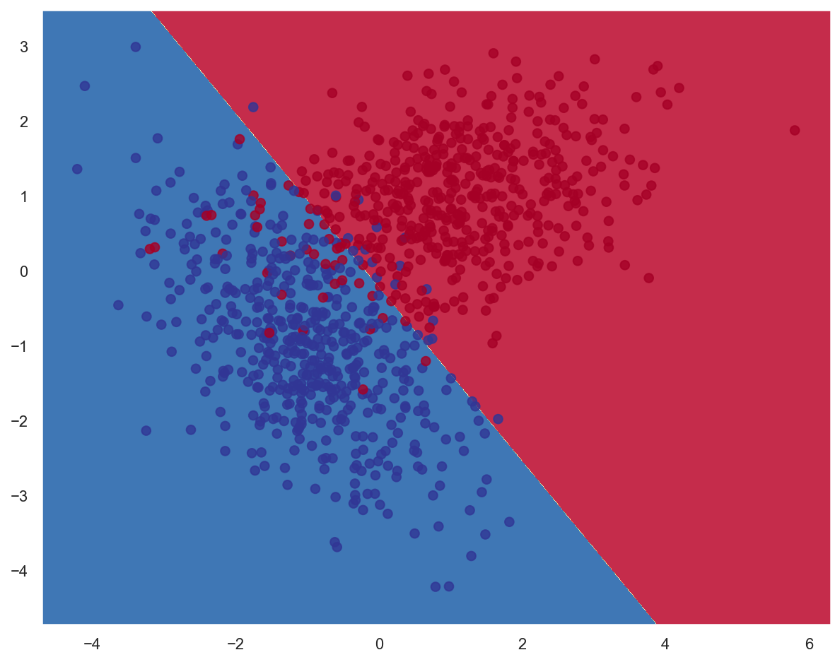
# Plot decision boundary
plot_decision_boundary(lambda x: lr_model.predict(x), x_train, y_train)
Multivariate regression
Problem formulation
Multivariate regression, also called softmax regression, is a generalization of logistic regression for multiclass classification.
A softmax regression model computes the scores \(s_k(\pmb{x})\) for each class \(k\), then estimates probabilities for each class by applying the softmax function to compute a probability distribution.
For a sample \(\pmb{x}^{(i)}\), the model predicts the class \(k\) that has the highest probability.
Each class \(k\) has its own parameter vector \(\pmb{\theta}^{(k)}\).
Model output
\(\pmb{y}^{(i)}\) (ground truth): binary vector of \(K\) values. \(y^{(i)}_k\) is equal to 1 if the \(i\)th sample’s class corresponds to \(k\), 0 otherwise.
\(\pmb{y}'^{(i)}\): probability vector of \(K\) values, computed by the model. \(y'^{(i)}_k\) represents the probability that the \(i\)th sample belongs to class \(k\).
Loss function: Categorical Crossentropy
See loss definition for details.
Model training
Via gradient descent:
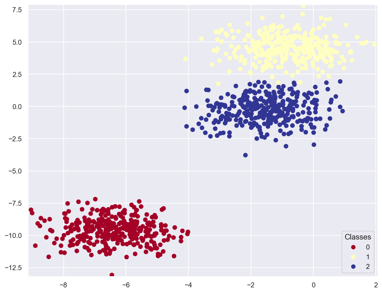
Example: classify multiclass planar data
# Generate 3 classes of linearly separable data
x_train_multi, y_train_multi = make_blobs(n_samples=1000, n_features=2, centers=3, random_state=11)

plot_data(x_train_multi, y_train_multi)
# Create a Logistic Regression model based on stochastic gradient descent
# Alternative: using LogisticRegression(multi_class="multinomial") which implements SR
lr_model_multi = SGDClassifier(loss="log")

# Train the model
lr_model_multi.fit(x_train_multi, y_train_multi)

print(f"Model weights: {lr_model_multi.coef_}, bias: {lr_model_multi.intercept_}")
Model weights: [[ -5.76624648 -17.43149458]
 [ -1.27339599  19.17812979]
 [  1.5231193   -0.91647832]], bias: [-133.15588019  -38.36388245    2.53712564]
# Print report with classification metrics
print(classification_report(y_train_multi, lr_model_multi.predict(x_train_multi)))
              precision    recall  f1-score   support

           0       1.00      1.00      1.00       334
           1       0.99      0.99      0.99       333
           2       0.99      0.99      0.99       333

    accuracy                           0.99      1000
   macro avg       0.99      0.99      0.99      1000
weighted avg       1.00      0.99      0.99      1000
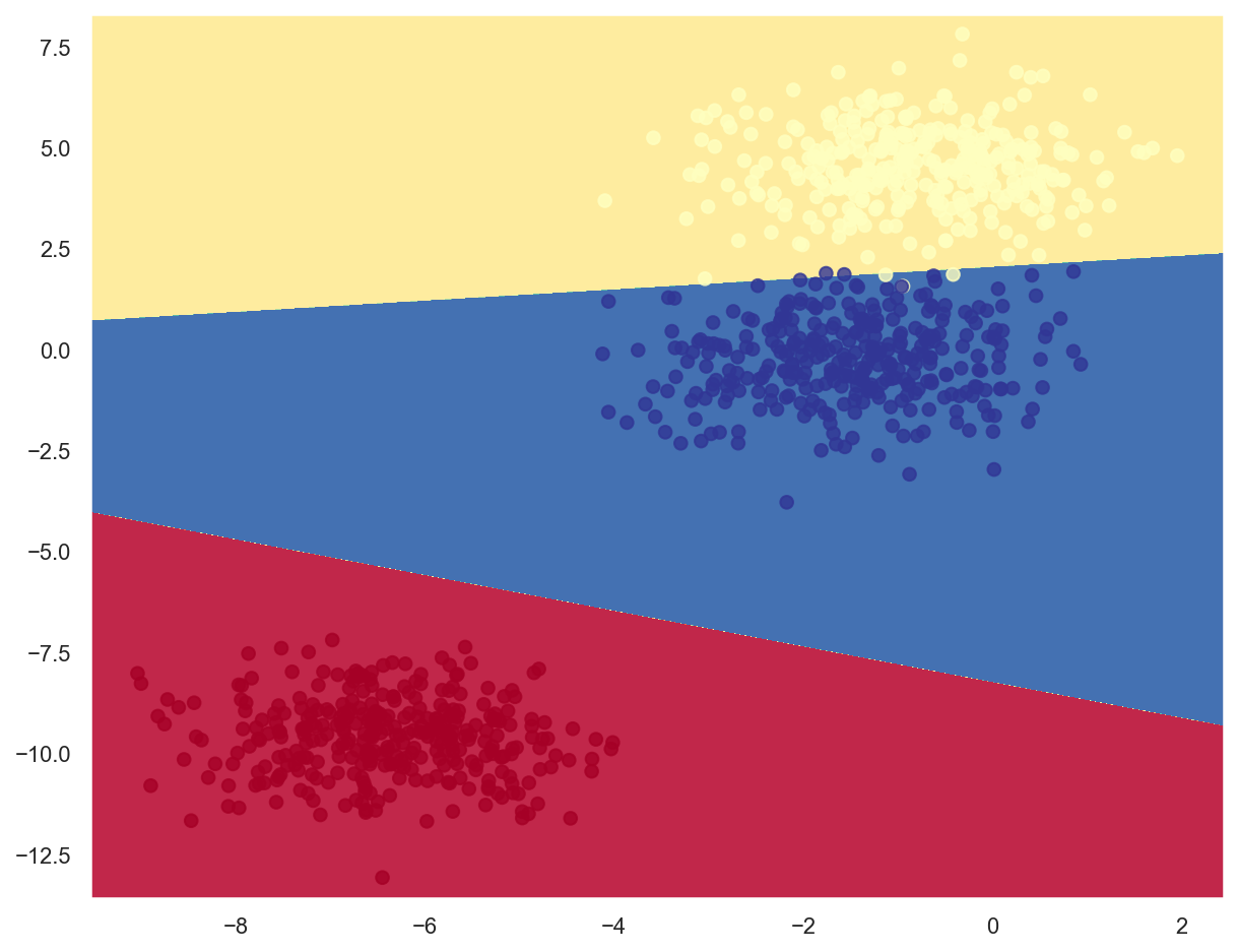
# Plot decision boundaries
plot_decision_boundary(lambda x: lr_model_multi.predict(x), x_train_multi, y_train_multi)
Titanic Disaster Survival Using Logistic Regression
#import libraries
import pandas as pd
import numpy as np
import seaborn as sns
import matplotlib.pyplot as plt
Load the Data
#load data
titanic_data=pd.read_csv('titanic_train.csv')
len(titanic_data)
891
View the data using head function which returns top rows
titanic_data.head()
| PassengerId | Survived | Pclass | Name | Sex | Age | SibSp | Parch | Ticket | Fare | Cabin | Embarked | |
|---|---|---|---|---|---|---|---|---|---|---|---|---|
| 0 | 1 | 0 | 3 | Braund, Mr. Owen Harris | male | 22.0 | 1 | 0 | A/5 21171 | 7.2500 | NaN | S |
| 1 | 2 | 1 | 1 | Cumings, Mrs. John Bradley (Florence Briggs Th... | female | 38.0 | 1 | 0 | PC 17599 | 71.2833 | C85 | C |
| 2 | 3 | 1 | 3 | Heikkinen, Miss. Laina | female | 26.0 | 0 | 0 | STON/O2. 3101282 | 7.9250 | NaN | S |
| 3 | 4 | 1 | 1 | Futrelle, Mrs. Jacques Heath (Lily May Peel) | female | 35.0 | 1 | 0 | 113803 | 53.1000 | C123 | S |
| 4 | 5 | 0 | 3 | Allen, Mr. William Henry | male | 35.0 | 0 | 0 | 373450 | 8.0500 | NaN | S |
titanic_data.index
RangeIndex(start=0, stop=891, step=1)
titanic_data.columns
Index(['PassengerId', 'Survived', 'Pclass', 'Name', 'Sex', 'Age', 'SibSp',
       'Parch', 'Ticket', 'Fare', 'Cabin', 'Embarked'],
      dtype='object')
titanic_data.info()
<class 'pandas.core.frame.DataFrame'>
RangeIndex: 891 entries, 0 to 890
Data columns (total 12 columns):
 #   Column       Non-Null Count  Dtype
---  ------       --------------  -----
 0   PassengerId  891 non-null    int64
 1   Survived     891 non-null    int64
 2   Pclass       891 non-null    int64
 3   Name         891 non-null    object
 4   Sex          891 non-null    object
 5   Age          714 non-null    float64
 6   SibSp        891 non-null    int64
 7   Parch        891 non-null    int64
 8   Ticket       891 non-null    object
 9   Fare         891 non-null    float64
 10  Cabin        204 non-null    object
 11  Embarked     889 non-null    object
dtypes: float64(2), int64(5), object(5)
memory usage: 83.7+ KB
titanic_data.dtypes
PassengerId      int64
Survived         int64
Pclass           int64
Name            object
Sex             object
Age            float64
SibSp            int64
Parch            int64
Ticket          object
Fare           float64
Cabin           object
Embarked        object
dtype: object
titanic_data.describe()
| PassengerId | Survived | Pclass | Age | SibSp | Parch | Fare | |
|---|---|---|---|---|---|---|---|
| count | 891.000000 | 891.000000 | 891.000000 | 714.000000 | 891.000000 | 891.000000 | 891.000000 |
| mean | 446.000000 | 0.383838 | 2.308642 | 29.699118 | 0.523008 | 0.381594 | 32.204208 |
| std | 257.353842 | 0.486592 | 0.836071 | 14.526497 | 1.102743 | 0.806057 | 49.693429 |
| min | 1.000000 | 0.000000 | 1.000000 | 0.420000 | 0.000000 | 0.000000 | 0.000000 |
| 25% | 223.500000 | 0.000000 | 2.000000 | 20.125000 | 0.000000 | 0.000000 | 7.910400 |
| 50% | 446.000000 | 0.000000 | 3.000000 | 28.000000 | 0.000000 | 0.000000 | 14.454200 |
| 75% | 668.500000 | 1.000000 | 3.000000 | 38.000000 | 1.000000 | 0.000000 | 31.000000 |
| max | 891.000000 | 1.000000 | 3.000000 | 80.000000 | 8.000000 | 6.000000 | 512.329200 |
Explaining Dataset
survival : Survival 0 = No, 1 = Yes
pclass : Ticket class 1 = 1st, 2 = 2nd, 3 = 3rd
sex : Sex
Age : Age in years
sibsp : Number of siblings / spouses aboard the Titanic
parch # of parents / children aboard the Titanic
ticket : Ticket number fare Passenger fare cabin Cabin number
embarked : Port of Embarkation C = Cherbourg, Q = Queenstown, S = Southampton
Data Analysis
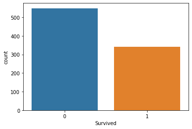
Import Seaborn for visually analysing the data, Find out how many survived vs Died using countplot method of seaboarn
#countplot of subrvived vs not survived
sns.countplot(x='Survived',data=titanic_data)
<AxesSubplot:xlabel='Survived', ylabel='count'>
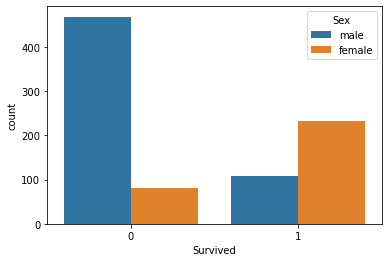
Male vs Female Survival
#Male vs Female Survived?
sns.countplot(x='Survived',data=titanic_data,hue='Sex')
<AxesSubplot:xlabel='Survived', ylabel='count'>
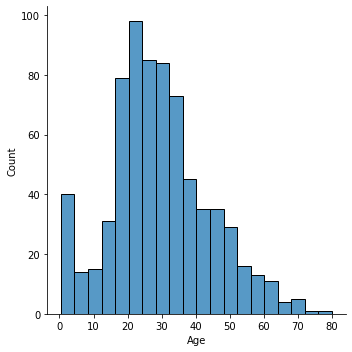
**See age group of passengeres travelled **
Note: We will use displot method to see the histogram. However some records does not have age hence the method will throw an error. In order to avoid that we will use dropna method to eliminate null values from graph
#Check for null
titanic_data.isna()
| PassengerId | Survived | Pclass | Name | Sex | Age | SibSp | Parch | Ticket | Fare | Cabin | Embarked | |
|---|---|---|---|---|---|---|---|---|---|---|---|---|
| 0 | False | False | False | False | False | False | False | False | False | False | True | False |
| 1 | False | False | False | False | False | False | False | False | False | False | False | False |
| 2 | False | False | False | False | False | False | False | False | False | False | True | False |
| 3 | False | False | False | False | False | False | False | False | False | False | False | False |
| 4 | False | False | False | False | False | False | False | False | False | False | True | False |
| ... | ... | ... | ... | ... | ... | ... | ... | ... | ... | ... | ... | ... |
| 886 | False | False | False | False | False | False | False | False | False | False | True | False |
| 887 | False | False | False | False | False | False | False | False | False | False | False | False |
| 888 | False | False | False | False | False | True | False | False | False | False | True | False |
| 889 | False | False | False | False | False | False | False | False | False | False | False | False |
| 890 | False | False | False | False | False | False | False | False | False | False | True | False |
891 rows × 12 columns
#Check how many values are null
titanic_data.isna().sum()
PassengerId      0
Survived         0
Pclass           0
Name             0
Sex              0
Age            177
SibSp            0
Parch            0
Ticket           0
Fare             0
Cabin          687
Embarked         2
dtype: int64
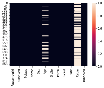
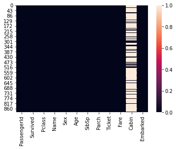
#Visualize null values
sns.heatmap(titanic_data.isna())
<AxesSubplot:>
#find the % of null values in age column
(titanic_data['Age'].isna().sum()/len(titanic_data['Age']))*100
19.865319865319865
#find the % of null values in cabin column
(titanic_data['Cabin'].isna().sum()/len(titanic_data['Cabin']))*100
77.10437710437711
#find the distribution for the age column
sns.displot(x='Age',data=titanic_data)
<seaborn.axisgrid.FacetGrid at 0x1509b6c8a30>
Data Cleaning
Fill the missing values
we will fill the missing values for age. In order to fill missing values we use fillna method.
For now we will fill the missing age by taking average of all age
#fill age column
titanic_data['Age'].fillna(titanic_data['Age'].mean(),inplace=True)
We can verify that no more null data exist
we will examine data by isnull mehtod which will return nothing
#verify null value
titanic_data['Age'].isna().sum()
0
Alternatively we will visualise the null value using heatmap
we will use heatmap method by passing only records which are null.
#visualize null values
sns.heatmap(titanic_data.isna())
<AxesSubplot:>
We can see cabin column has a number of null values, as such we can not use it for prediction. Hence we will drop it
#Drop cabin column
titanic_data.drop('Cabin',axis=1,inplace=True)
#see the contents of the data
titanic_data.head()
| PassengerId | Survived | Pclass | Name | Sex | Age | SibSp | Parch | Ticket | Fare | Embarked | |
|---|---|---|---|---|---|---|---|---|---|---|---|
| 0 | 1 | 0 | 3 | Braund, Mr. Owen Harris | male | 22.0 | 1 | 0 | A/5 21171 | 7.2500 | S |
| 1 | 2 | 1 | 1 | Cumings, Mrs. John Bradley (Florence Briggs Th... | female | 38.0 | 1 | 0 | PC 17599 | 71.2833 | C |
| 2 | 3 | 1 | 3 | Heikkinen, Miss. Laina | female | 26.0 | 0 | 0 | STON/O2. 3101282 | 7.9250 | S |
| 3 | 4 | 1 | 1 | Futrelle, Mrs. Jacques Heath (Lily May Peel) | female | 35.0 | 1 | 0 | 113803 | 53.1000 | S |
| 4 | 5 | 0 | 3 | Allen, Mr. William Henry | male | 35.0 | 0 | 0 | 373450 | 8.0500 | S |
Preaparing Data for Model
No we will require to convert all non-numerical columns to numeric. Please note this is required for feeding data into model. Lets see which columns are non numeric info describe method
#Check for the non-numeric column
titanic_data.info()
<class 'pandas.core.frame.DataFrame'>
RangeIndex: 891 entries, 0 to 890
Data columns (total 11 columns):
 #   Column       Non-Null Count  Dtype
---  ------       --------------  -----
 0   PassengerId  891 non-null    int64
 1   Survived     891 non-null    int64
 2   Pclass       891 non-null    int64
 3   Name         891 non-null    object
 4   Sex          891 non-null    object
 5   Age          891 non-null    float64
 6   SibSp        891 non-null    int64
 7   Parch        891 non-null    int64
 8   Ticket       891 non-null    object
 9   Fare         891 non-null    float64
 10  Embarked     889 non-null    object
dtypes: float64(2), int64(5), object(4)
memory usage: 76.7+ KB
titanic_data.dtypes
PassengerId      int64
Survived         int64
Pclass           int64
Name            object
Sex             object
Age            float64
SibSp            int64
Parch            int64
Ticket          object
Fare           float64
Embarked        object
dtype: object
We can see, Name, Sex, Ticket and Embarked are non-numerical.It seems Name,Embarked and Ticket number are not useful for Machine Learning Prediction hence we will eventually drop it. For Now we would convert Sex Column to dummies numerical values****
#convert sex column to numerical values
gender=pd.get_dummies(titanic_data['Sex'],drop_first=True)
titanic_data['Gender']=gender
titanic_data.head()
| PassengerId | Survived | Pclass | Name | Sex | Age | SibSp | Parch | Ticket | Fare | Embarked | Gender | |
|---|---|---|---|---|---|---|---|---|---|---|---|---|
| 0 | 1 | 0 | 3 | Braund, Mr. Owen Harris | male | 22.0 | 1 | 0 | A/5 21171 | 7.2500 | S | 1 |
| 1 | 2 | 1 | 1 | Cumings, Mrs. John Bradley (Florence Briggs Th... | female | 38.0 | 1 | 0 | PC 17599 | 71.2833 | C | 0 |
| 2 | 3 | 1 | 3 | Heikkinen, Miss. Laina | female | 26.0 | 0 | 0 | STON/O2. 3101282 | 7.9250 | S | 0 |
| 3 | 4 | 1 | 1 | Futrelle, Mrs. Jacques Heath (Lily May Peel) | female | 35.0 | 1 | 0 | 113803 | 53.1000 | S | 0 |
| 4 | 5 | 0 | 3 | Allen, Mr. William Henry | male | 35.0 | 0 | 0 | 373450 | 8.0500 | S | 1 |
#drop the columns which are not required
titanic_data.drop(['Name','Sex','Ticket','Embarked'],axis=1,inplace=True)
titanic_data.head()
| PassengerId | Survived | Pclass | Age | SibSp | Parch | Fare | Gender | |
|---|---|---|---|---|---|---|---|---|
| 0 | 1 | 0 | 3 | 22.0 | 1 | 0 | 7.2500 | 1 |
| 1 | 2 | 1 | 1 | 38.0 | 1 | 0 | 71.2833 | 0 |
| 2 | 3 | 1 | 3 | 26.0 | 0 | 0 | 7.9250 | 0 |
| 3 | 4 | 1 | 1 | 35.0 | 1 | 0 | 53.1000 | 0 |
| 4 | 5 | 0 | 3 | 35.0 | 0 | 0 | 8.0500 | 1 |
#Seperate Dependent and Independent variables
x=titanic_data[['PassengerId','Pclass','Age','SibSp','Parch','Fare','Gender']]
y=titanic_data['Survived']
y
0      0
1      1
2      1
3      1
4      0
      ..
886    0
887    1
888    0
889    1
890    0
Name: Survived, Length: 891, dtype: int64
Data Modelling
Building Model using Logestic Regression
Build the model
#import train test split method
from sklearn.model_selection import train_test_split
#train test split
x_train, x_test, y_train, y_test = train_test_split(x, y, test_size=0.33, random_state=42)
#import Logistic Regression
from sklearn.linear_model import LogisticRegression
#Fit Logistic Regression
lr=LogisticRegression()
lr.fit(x_train,y_train)
C:\Users\gggg\anaconda3\lib\site-packages\sklearn\linear_model\_logistic.py:762: ConvergenceWarning: lbfgs failed to converge (status=1):
STOP: TOTAL NO. of ITERATIONS REACHED LIMIT.

Increase the number of iterations (max_iter) or scale the data as shown in:
    https://scikit-learn.org/stable/modules/preprocessing.html
Please also refer to the documentation for alternative solver options:
    https://scikit-learn.org/stable/modules/linear_model.html#logistic-regression
  n_iter_i = _check_optimize_result(
LogisticRegression()
#predict
predict=lr.predict(x_test)
Testing
See how our model is performing
#print confusion matrix
from sklearn.metrics import confusion_matrix
pd.DataFrame(confusion_matrix(y_test,predict),columns=['Predicted No','Predicted Yes'],index=['Actual No','Actual Yes'])
| Predicted No | Predicted Yes | |
|---|---|---|
| Actual No | 151 | 24 |
| Actual Yes | 37 | 83 |
#import classification report
from sklearn.metrics import classification_report
print(classification_report(y_test,predict))
              precision    recall  f1-score   support

           0       0.80      0.86      0.83       175
           1       0.78      0.69      0.73       120

    accuracy                           0.79       295
   macro avg       0.79      0.78      0.78       295
weighted avg       0.79      0.79      0.79       295
Precision is fine considering Model Selected and Available Data. Accuracy can be increased by further using more features (which we dropped earlier) and/or by using other model
Note:
Precision : Precision is the ratio of correctly predicted positive observations to the total predicted positive observations
Recall : Recall is the ratio of correctly predicted positive observations to the all observations in actual class
F1 score - F1 Score is the weighted average of Precision and Recall.