2. EDA

上一章我们了解了GAN的概念、模型以及评价指标。在本章中，我们将检查实践中使用的数据集。

在 GAN 教程中，我们将构建一个模型将黑白图像转换为彩色图像。用于构建模型的数据集称为Victorian400 Victorian400，它是由 19 世纪绘画的黑白/彩色对组成的数据。我们将使用这些数据构建彩色图像生成模型，并输入新的黑白图像来检查着色性能。

Victorian400数据由400张黑白和彩色图片组成。由于数据集数量合适，训练模型不需要较长的时间，适合体验GAN学习过程的数据。在练习了使用数据训练 GAN 模型的整个过程后，我们建议您将 GAN 应用于适合您需求的其他数据。

在 2.1 节中，我们将了解如何下载数据。在第 2.2 节中，我们将可视化数据，在第 2.3 节中，我们将学习如何使用matplotlib.pyplot提供的函数在一个输出窗口中可视化多个图像。subplots最后，在2.4节中，我们将通过图像预处理对像素值进行归一化。

2.1 数据集下载

!git clone https://github.com/Pseudo-Lab/Tutorial-Book-Utils

'git' 不是内部或外部命令，也不是可运行的程序
或批处理文件。

首先使用命令复制公共Github仓库并保存到Colab环境中。执行上述代码后，会创建一个如图2-1所示的文件夹。git cloneTutorial-Book-Utils

• 图2-1 使用git clone命令后的文件夹结构

我们PL_data_loader.py将使用该文件夹中的文件下载用于构建模型的数据集。将使用以下命令执行下载。

!python Tutorial-Book-Utils/PL_data_loader.py --data GAN-Colorization

python: can't open file 'D:\3000-code\deeplearning\DeepLearning2023\Deeplearning\chapters\chpt3\Tutorial-Book-Utils\PL_data_loader.py': [Errno 2] No such file or directory

下载完成后，Victorian400-GAN-colorization-data.zip将创建一个文件，如图2-2所示。unzip我们将使用该命令来解压缩压缩文件。

• 图2-2 运行PL_data_loader.py后的文件夹结构

!unzip -q Victorian400-GAN-colorization-data.zip

'unzip' 不是内部或外部命令，也不是可运行的程序
或批处理文件。

解压后会生成文件夹gray、original、resized，如图2-3所示。该文件夹中保存尺寸为256×256的黑白图像，该文件夹中保存尺寸为256×256的彩色图像。彩色图像以其原始尺寸存储在文件夹中。该文件夹包含六对黑白和彩色图像，用于评估模型性能。为了构建模型，我们将仅使用和文件夹中的图像。testgrayresizedoriginaltestgrayresized

• 图2-3 执行unzip后的文件夹结构

2.2 检查数据集¶

2.1让我们可视化第 2.1 节中下载的数据并检查存储了哪些图像。首先，让我们加载必要的库。os和globlibrary在处理文件夹路径时使用，matplotliblibrary是用于可视化的代表性库。cv2是处理图像文件时使用的库。

import os
import glob
import matplotlib.pyplot as plt
import cv2

接下来，os.listdir()让我们使用该函数来检查original、resized、 和文件gray夹中存储了多少张图像。

origin_dir = 'original/'
resized_dir = 'resized/'
gray_dir = 'gray/'

print('number of files in "original" folder:', len(os.listdir(origin_dir)))
print('number of files in "resized" folder:', len(os.listdir(resized_dir)))
print('number of files in "gray" folder:', len(os.listdir(gray_dir)))

---------------------------------------------------------------------------
FileNotFoundError                         Traceback (most recent call last)
Cell In[5], line 5
      2 resized_dir = 'resized/'
      3 gray_dir = 'gray/'
----> 5 print('number of files in "original" folder:', len(os.listdir(origin_dir)))
      6 print('number of files in "resized" folder:', len(os.listdir(resized_dir)))
      7 print('number of files in "gray" folder:', len(os.listdir(gray_dir)))

FileNotFoundError: [WinError 3] 系统找不到指定的路径。: 'original/'

您可以看到每个保存了 400 张图像。接下来，test让我们检查文件夹结构以及该文件夹中存储的图像数量。

test_dir = 'test/'

print(os.listdir(test_dir))
print('number of files in "test/gray" folder:', len(os.listdir(test_dir + 'gray')))
print('number of files in "test/resized" folder:', len(os.listdir(test_dir + 'resized')))

['resized', 'gray']
number of files in "test/gray" folder: 6
number of files in "test/resized" folder: 6

test里面有gray文件夹和resized文件夹。可以看到每个文件夹中保存了6张图片。

现在我们已经确认了每个文件夹中存储的图像数量，让我们可视化并检查每个图像。test让我们首先可视化除该文件夹之外的所有文件夹中存在的图像。为了形象化，我们将每个文件的路径保存在一个变量中。origin文件夹内的图像路径将存储origin_files在变量中，resized文件夹内的图像路径将存储resized_files在变量中，gray文件夹内的图像路径gray_files将存储在变量中。

origin_files = sorted(glob.glob(origin_dir + '*'))
resized_files = sorted(glob.glob(resized_dir + '*'))
gray_files = sorted(glob.glob(gray_dir + '*'))

让我们检查一下为每个变量存储的两个值。

print(origin_files[:2])

print(resized_files[:2])

print(gray_files[:2])

['original/Victorian1.png', 'original/Victorian10.png']
['resized/Victorian1.png', 'resized/Victorian10.png']
['gray/Victorian1.png', 'gray/Victorian10.png']

[폴더명]_files您可以看到位于该文件夹中的图像文件的路径保存在变量中。Victorian1.png原始图像original保存在该文件夹中，调整大小为 256 x 256 的图像resized保存在 中，黑白图像gray保存在该文件夹中。

接下来， 我们将使用cv2.imread()函数和plt.imshow()函数将每个文件夹中存储的图像一一可视化。首先，read_img()我们定义一个读取图像的函数。该函数cv2.imread()使用函数BGR以数组的形式读取图像的值。存储cv2.imread()读入的数组img_arr后cv2.cvtColor，使用该函数将BGR值更改为某个值。RGB让我们plt.imshow()使用函数将该值表达为图像。

# 使用cv2模块定义读取图像的函数
def read_img(file_path):
    img_arr = cv2.imread(file_path)
    return cv2.cvtColor(img_arr, cv2.COLOR_BGR2RGB)

img_arr = read_img(origin_files[0])

# 输出文件路径
print(origin_files[0])

# 输出图像大小
print(img_arr.shape)

# 图像可视化
plt.imshow(img_arr)

original/Victorian1.png
(714, 750, 3)

<matplotlib.image.AxesImage at 0x7f1d7768ce10>

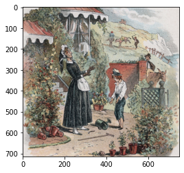
original Victorian1.png您可以看到该文件夹​​中保存了一张尺寸为 714 x 750 的图像。

img_arr = read_img(resized_files[0])

# 输出文件路径
print(resized_files[0])

# 输出图像大小
print(img_arr.shape)

# 图像可视化
plt.imshow(img_arr)

resized/Victorian1.png
(256, 256, 3)

<matplotlib.image.AxesImage at 0x7f1d7588f0b8>

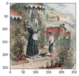
resized Victorian1.png您可以看到该文件夹​​中保存了一张尺寸为 256 x 256 的图像。

img_arr = read_img(gray_files[0])

# 输出文件路径
print(gray_files[0])

# 输出图像大小
print(img_arr.shape)

# 图像可视化
plt.imshow(img_arr)

gray/Victorian1.png
(256, 256, 3)

<matplotlib.image.AxesImage at 0x7f1d75870710>

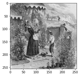
gray 的 Victorian1.png您可以看到该文件夹​​中保存了一张尺寸为 256 x 256 的黑白图像。

我们比较了每个文件夹中存储的图像。然而，由于一幅图像在一个输出单元中可视化，因此比较多幅图像是有限的。因此，在下一节中，plt.subplots()我们将使用该函数将多个图像输出到一个输出窗口并进行比较。

2.3 使用 plt.subplots() 可视化

我们将从每个文件夹中img_num读取图像数量img_arrs并将它们保存在 .使用下面的代码original，我们将从resized、 和文件夹中各读取五张图像。gray

img_arrs = []

img_num = 5

for idx in range(img_num):
    
    img_arrs.append(read_img(origin_files[idx]))
    img_arrs.append(read_img(resized_files[idx]))
    img_arrs.append(read_img(gray_files[idx]))

len(img_arrs)

15

由于从 3 个文件夹中各读取了 5 张图像，因此总共 15 张图像img_arrs保存在 .

接下来，plt.subplots()我们使用该函数将 15 张图像输出到一个输出窗口。该函数接收以下三个参数作为输入。

nrows：显示图像板的行数

ncols：显示图像板中的列数

figsize：（水平、垂直）每张图像的尺寸

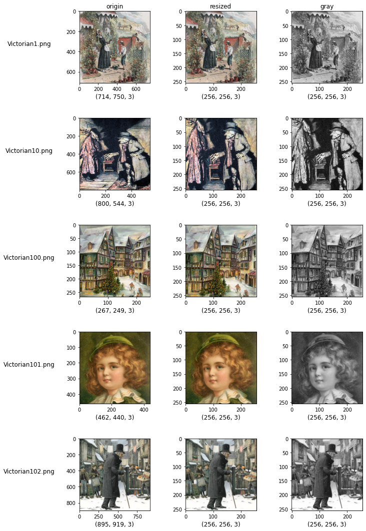
由于我们有15 个图像img_arrs存储在变量中，因此让我们在 5 行 3 列的图像板上将它们可视化

rows = img_num
columns = 3


# 设置画布
fig, axes = plt.subplots(nrows=rows, ncols=columns, figsize=(columns*3, rows*3))

# 在每个子图中显示图像
for num in range(1, rows*columns+1): # 从1号到15号
    
    fig.add_subplot(rows, columns, num) # 输入想要的位置编号(num)
    
    idx = num - 1
    
    plt.imshow(img_arrs[idx], aspect='auto')
    plt.xlabel(f'{img_arrs[idx].shape}', fontsize=12)

fig.tight_layout() # 调整图像之间的间距

for file_idx, ax in enumerate(axes[:,0]): # 对第一列的图像进行循环
    ax.set_ylabel(f'{sorted(os.listdir(origin_dir))[file_idx]}',  # 使用文件名作为y轴标签
                rotation=0,
                fontsize=12,
                labelpad=100) # 调整y轴与标签之间的间距

cols = ['origin', 'resized', 'gray']

# 设置标题
for folder_idx, ax in enumerate(axes[0]):
    ax.set_title(cols[folder_idx])

# 移除xtick和ytick
for idx, ax in enumerate(axes.flat):
    ax.set_xticks([])
    ax.set_yticks([])

我们来一一看代码。plt.subplots()该函数创建一个大小为nrowsx的网格。ncols上面的代码创建了一个 5 行 3 列的画笔。每个网格中的每个单元格都会分配一个唯一的编号。数字从 1 到 15 ( nrowsx )。ncols编号是从左到右、从上到下分配的。如图2-4所示，数字1、2、3从第一行左侧单元格开始分配，数字4、5、6从第二行左侧单元格开始分配。

• 图 2.4 分配给每个网格单元的数字

要将图像添加到每个单元格，add_subplot()请使用函数选择单元格。然后plt.show()使用该函数可视化所选单元格上的图像。此时，设置aspect参数auto即可自动调整图像的长宽比。另外，plt.xlabel()我们使用一个函数在x轴上显示每个图像的大小。

接下来，fig.tight_layout()使用该功能调整图像之间的间距。

打印的网格涂料的每一行包含每个图像，每一列代表保存图像的文件夹。我们会将文件名和文件夹名称与图像一起打印，以便您直观地看到内容。

axes包含15个细胞的图像信息。set_ylabel()使用该功能仅选择第一列中保存的图像，并将图像的文件名记录为 y 轴名称。另外，仅选择第一行中保存的图像，并按顺序输入original、resized、 和作为图像标题。gray

最后，xticks去除每张图像中的yticks, 并输出最终结果。根据上述结果，您可以在一个输出窗口中比较 15 个图像。original可以看到文件夹中以各种尺寸保存了彩色图像，resized而gray在 和 文件夹中可以看到尺寸为256 x 256的图像分别以彩色和黑白格式保存。

2.4 图像预处理

在本节中，我们将执行图像预处理。在获得400张resized图像和gray图像的每个通道的平均值和标准差值后，我们将通过减去每个图像像素的平均值然后除以标准差来进行归一化。理论上，归一化图像可以帮助神经网络模型更快地收敛。我们将定义一个函数来计算所有图像的平均值和标准偏差，get_mean_and_std()如下所示。

import numpy as np

def get_mean_and_std(files):
    # global mean 구하기
    global_mean = 0
    global_var = 0

    for img in files:
        img_arr = read_img(img) / 255
        global_mean += img_arr.reshape(-1, 3).mean(axis=0)

    global_mean /= len(files)

    # global std 구하기
    for img in files:
        img_arr = read_img(img) / 255
        global_var += ((img_arr.reshape(-1, 3) - global_mean)**2).mean(axis=0)
    
    global_var /= len(files)
    global_std = np.sqrt(global_var)

    return global_mean, global_std

在计算平均值和标准差值之前，我们将像素值除以255，将像素值的范围转换为0到1之间，然后计算值。这样做的原因是，在第3章和第4章中，transforms.ToTensor()我们计划使用函数将图像转换为张量形式，而此时，transforms.ToTensor()由于函数的性质，像素值在0和1之间转换。因此，我们会得到像素值在0到1范围内时的平均值和标准差值，以便用于后面的归一化。

将每幅图像的平均值累加并相加，然后len(files)除以包含图像总数的数字以计算所有图像的平均值。求整个图像的标准差，就是用像素值减去之前计算的平均值得到偏差，然后计算偏差平方值的平均值，首先计算整个图像像素值的方差。然后，我们取方差的根来找到标准差。

您可以使用如下所示的方式定义的函数get_mean_and_std()来查找彩色图像和黑白图像的平均值和标准差。

# 调用 get_mean_and_std 函数计算调整大小后的图像的均值和标准差
color_mean, color_std = get_mean_and_std(resized_files)
# 输出计算得到的均值和标准差
color_mean, color_std

(array([0.58090717, 0.52688643, 0.45678478]),
 array([0.25644188, 0.25482641, 0.24456465]))

# 调用 get_mean_and_std 函数计算灰度图像的均值和标准差
gray_mean, gray_std = get_mean_and_std(gray_files)
# 输出计算得到的均值和标准差
gray_mean, gray_std

(array([0.5350533, 0.5350533, 0.5350533]),
 array([0.25051587, 0.25051587, 0.25051587]))

我们来比较一下标准化前后的差异。首先，读取新图像并将其除以255，将像素值转换为0和1之间

color_img = read_img(resized_files[0]) / 255
gray_img = read_img(gray_files[0]) / 255

RGBget_statistics我们将定义一个函数，以便我们可以检查每个通道的统计数据。该函数RGB返回每个通道的平均值、标准差、最小值和最大值等统计值。您可以使用pandas库提供的pd.DataFrame.describe()函数轻松计算统计值。

import pandas as pd

def get_statistics(arr):
    return pd.DataFrame(arr.reshape(-1, 3), columns=["R", "G", "B"]).describe()

color_img我们来看看 的统计值。

get_statistics(color_img)

	R	G	B
count	65536.000000	65536.000000	65536.000000
mean	0.564941	0.537205	0.493146
std	0.208751	0.203116	0.198431
min	0.027451	0.039216	0.058824
25%	0.411765	0.380392	0.333333
50%	0.584314	0.533333	0.478431
75%	0.745098	0.709804	0.650980
max	0.929412	0.913725	0.909804

可以看到最小值和最大值分布在0和1之间。接下来gray_img我们来看看 的统计值。.

get_statistics(gray_img)

	R	G	B
count	65536.000000	65536.000000	65536.000000
mean	0.540488	0.540488	0.540488
std	0.201794	0.201794	0.201794
min	0.047059	0.047059	0.047059
25%	0.388235	0.388235	0.388235
50%	0.541176	0.541176	0.541176
75%	0.713725	0.713725	0.713725
max	0.917647	0.917647	0.917647

由于是黑白图像，所以所有通道的值都是相同的，所以可以看到每个通道的统计值也是相同的。接下来，让我们检查一下get_mean_and_std()通过函数 计算出的color_mean、color_std、gray_mean、gray_std归一化后的统计值。分别将标准化值存储在normalized_color_img中。normalized_gray_img

normalized_color_img = (color_img - color_mean) / color_std
normalized_gray_img = (gray_img - gray_mean) / gray_std

get_statistics()让我们使用该函数来计算每个通道的统计数据normalized_color_img。RGB

get_statistics(normalized_color_img)

	R	G	B
count	65536.000000	65536.000000	65536.000000
mean	-0.062259	0.040491	0.148678
std	0.814030	0.797075	0.811364
min	-2.158213	-1.913737	-1.627223
25%	-0.659574	-0.574879	-0.504780
50%	0.013284	0.025299	0.088511
75%	0.640265	0.717812	0.794046
max	1.359000	1.518049	1.852349

标准化后，您可以看到均值已转换为接近 0，标准差已转换为接近 1。之所以不完全是0和1，是因为归一化时使用的均值和标准差不是从单个图像获得的值，而是使用整个数据集获得的值。

get_statistics(normalized_gray_img)

	R	G	B
count	65536.000000	65536.000000	65536.000000
mean	0.021694	0.021694	0.021694
std	0.805516	0.805516	0.805516
min	-1.947958	-1.947958	-1.947958
25%	-0.586063	-0.586063	-0.586063
50%	0.024442	0.024442	0.024442
75%	0.713217	0.713217	0.713217
max	1.527224	1.527224	1.527224

同样，normalized_gray_img平均值转换为 0，标准差转换为接近 1。

到目前为止，我们已经可视化了 Victorian400 数据集中存储的图像。在第 3 章中，我们将构建一个 GAN 模型，使用 Victorian400 数据集将黑白图像转换为彩色图像。